Super VRT

This article This paper presents a method for VSR A parallel superpartition model based on ——VRT.VRT It's a use of Vision-Transformer To model feature propagation , At its core is a Temporal Mutual Self Attention(TMSA) modular —— Will be based on swin-T Of Mutual-Attention and Self-Attention To extract or aggregate the local and global feature information of video sequences by fusion , And use the flow-guided DCN Alignment Of Parallel Warping(PW) To align , And fuse the adjacent frames , Finally, the video sequence up sampling is completed by the reconstruction module . Besides ,VRT Used 4 Different scales (multi-scale) To extract the characteristic information of different receptive fields , For smaller resolution, you can capture larger motion to better align large motion , For larger resolution, it is more conducive to capture more local correlation and aggregate local information .

Note：

1. VRT It can be applied to many video recovery tasks , Such as super score 、 Denoise 、 To blur 、 Go to a task, etc , But this article only aims at analyzing video hyperanalysis VSR part .
2. VRT and VSRT The same authors .
3. Personal opinion ： This article seems to be the feeling of piling up some junk , Hard learning with larger models $LR\to HR$.

Reference list ：
① Source code

Abstract

1. since VSRT after ,VSR The fields can be roughly divided into 3 class ：①Sliding-windows;②Recurrent;③Vision-Transformer. Sliding windows local Can not capture feature information over a long distance ; And based on RNN Of VSR Method can only perform frame by frame reconstruction serially . Therefore, in order to solve the above 2 A question , The author puts forward It has the ability to capture the global correlation over a long distance , It can also realize frame parallel reconstruction , This is it. VRT Model .
2. VRT It consists of many scales , Each scale is called 1 individual stage, In the experiment, a total of 8 individual stage. front 7 Each of the three scales consists of 1 individual TMSA Group (TMSAG) concatenated 1 individual Parallel Warping(PW); The first 8 individual stage( namely RTMSA) Only by 1 individual TMSAG form , But it doesn't include PW. Besides ,1 individual TMSA from $depth$ individual TMSA The modules are connected in series ; And each TMSA A module is Transformer Of Encoder part , The attention part is made up of 1 individual Multi-head Mutual Attention and 1 individual Multi-head Self Attention form ; and FFN Is used GEGLU Instead of .
3. In order to reduce the VSRT A lot of similarity computation in time and space ,VRT be based on Swin-Transformer, That is, to gather the local correlation in the form of windowing . differ Swin-IR,VRT My window is 3 Dimension window , Time + Space , For example, in the experiment $(2,8,8)$ The window of , In the time dimension 2 Frame by frame , Spatially, with $8\times 8$ Split the units , Therefore, the calculation of similarity is $2\times 8\times 8$ individual token Between . And all the windows are put in Batch dimension , so Every window is GPU Do calculations in parallel and independently of each other .
4. Whether it's Self attention or mutual attention (mutual-attention), It's all based on 3D Window , Not the whole image . Suppose the window is $(2,8,8)$, Then self attention is the same as VSRT equally , stay $2\times 8\times 8$ individual token Do self attention in time and space ; and mutual-attention It is in 2 Respective... On the frame 2D Do mutual attention between windows . But such a feature transmission mode will be limited to 2 Within the frame , So the author draws lessons from swin-T At the heart of ——shifting Thought , Set up 3D Move the window $(2/2,8/2,8/2)=(1,4,4)$ Move in space and time .
5. Self attention is used to extract feature information in space and time , Mutual attention is used for feature alignment , This idea is the same as TTVSR The trajectory of attention is the same .
6. VSRT The alignment of can be said to be parallel , Because he put the frame in batch dimension ; however VRT The alignment of the antecedent and antecedent branches is actually serial , adopt for Circular .PW The process of integration and VSRT It's the same —— The two branches are aligned separately , Last 2 The alignment results of the branches are fused with the reference frame sequence , In terms of its fusion nature , In fact, the time window is 3 When the sliding-windows Alignment mode ——$[f_{t-1}\to f_t;f_{t+1}\to f_t]$;PW It uses optical flow guidance DCN Alignment method .
7. VRT At present, it is No. 1 in the ranking list , made SOTA Expressive force .

Note：

1. Optical flow through SpyNet obtain , and TTVSR equally , about $n$ frame , Study $n-1$ An optical flow ; and VSRT Is learning $n$ An optical flow . Here is a schematic diagram of optical flow estimation ：

2. In the source code, the author uses $64\times 64$ by patch size , use $64、32、16、8$ common 4 Three resolution scales .

3. VRT Key points of ：① Overall architecture design ;②TMSA;③PW;④windows&shifting-windows;⑤multi-scale.

1 Introduction

The picture above shows 3 A way of characteristic transmission , From left to right are Silding-windows、Recurrent、VRT( It can also be used as Transformer Class ).

$Silding-windows$：
This way is VSR Typical early methods , The time window ( Or the size of time 、 Time feels wild 、 Time filter ) Fixed for 3、5 or 7 frame , Typical representative VESPCN、TDAN、Robust-LTD、EDVR etc. . One of the drawbacks of this method is that the available feature information is relatively limited , Only... Can be used for each alignment local Frame information of ; Second, in the whole training process , The same frame is treated as a support frame multiple times , It may be repeated many times from the beginning , This will result in unnecessary computational costs , It is a relatively inefficient way of using feature information .

$Recurrent$
This way is to VSR Modeling as Seq2Seq The way , Each time you align, you should use the alignment results of the previous frame to help align the current frame , because RNN The hidden state of the structure can remember the past information , Therefore, it can be said to use all the characteristic information of the past or the future , Typical representative BasicVSR series (BasicVSR、BasicVSR++)、RLSP etc. . One of the drawbacks of this method is that it is easy to produce gradient vanishing phenomenon in long sequences , As a result, far away feature information is not captured ( This is a RNN The defects of ); Second, it is prone to error accumulation and information attenuation , This is because one frame may have a great impact on the next frame , But it will spread for a while , This information will be of little help to the next frame , Because in the process of transmission , The hidden state is constantly refreshed ; Third, it is difficult to produce high performance in short sequence video , This is in VSRT It has been proved in the experiment of ; Fourth, this method is used to reconstruct frame by frame , Parallel processing is not possible .

$Vision-Transformer$
since Recurrent take VSR Modeling as Seq2Seq problem , Then based on RNN Over to Transformer, And we can extract appropriate feature information from long sequences according to the attention mechanism to help alignment . Based on this idea ,2021 year VSRT It was born , It can extract feature information in parallel , Parallel alignment . But the flaw is token Too many , Need to consume too much computing resources , This also limits its application to larger LRS.VRT This is the parallel model , It can do parallel computing , And capture the correlation over a long distance , This long distance includes the spatial dimension , It also includes the time dimension . Now, there have been a lot of papers based on Vision-Transformer Of VSR Method , It mainly optimizes the calculation amount 、 How to capture the feature information of a longer sequence , Such as TTVSR And how to further gather better local information .

---

Next, let's talk about VRT Give a brief introduction .
①VRT Network structure ：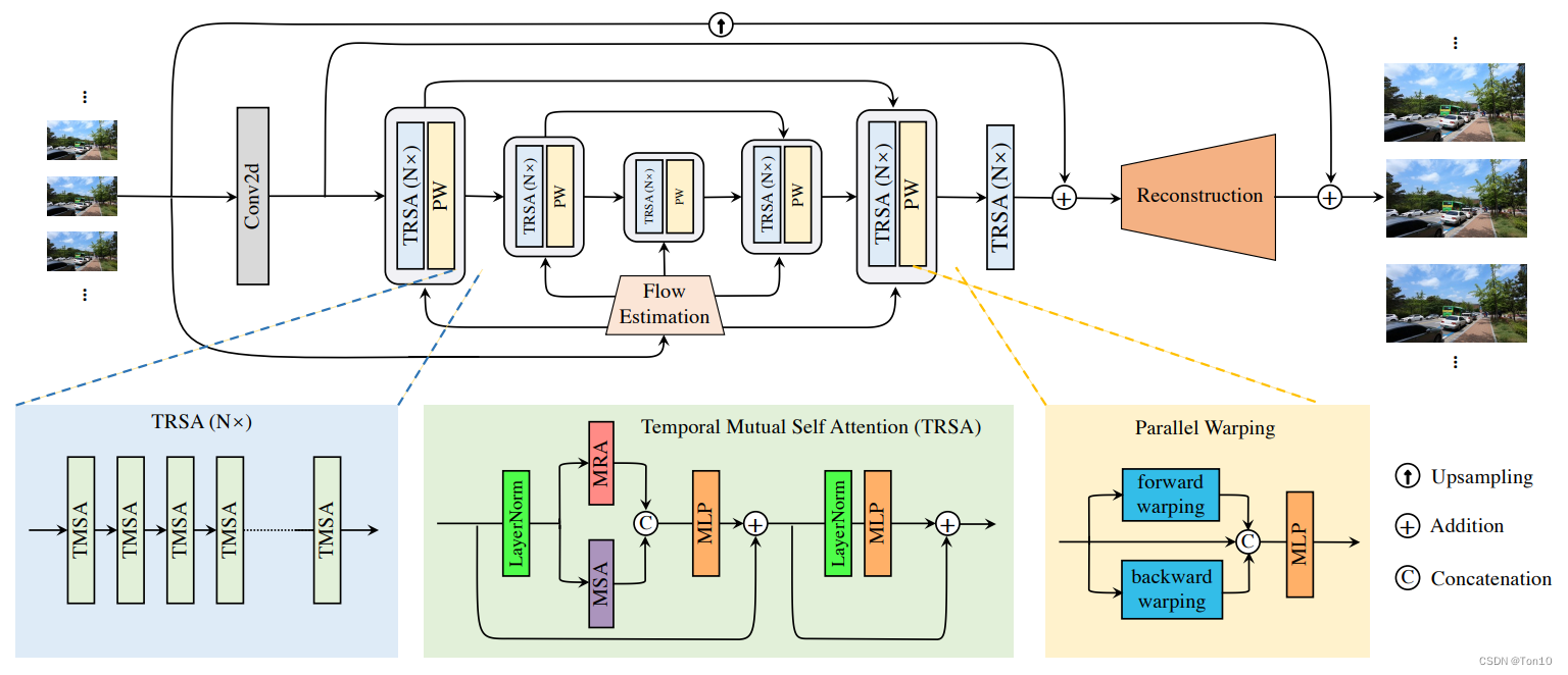

VRT Of pipeline It is composed of multiple scale blocks connected in series , Each scale block is mainly used based on windows Feature alignment and feature extraction ; At the end of each block, there is also a DCN-based Align blocks , We call each block stage.
VRT Of 8 individual stage After that, we can do SR Supersession reconstruction , In order to make the reconstruction work in parallel , Use 3D Convolution +pixelshuffle The way to do it ( See Section III for detailed analysis ).

②Multi-scale：
VSR The reconstruction needs to combine feature extraction and alignment of multiple receptive fields or multiple resolution scales , Therefore, it is necessary to set a certain number of scales . In the experiment 4 Three resolution scales ——$64\times 64、32\times 32、16\times 16、8\times 8$, Because the window size of each scale is the same , therefore $16\times 16$ Although the resolution is low , But in every window token The feeling field is bigger , It is more convenient to deal with the alignment of large motion ; and $64\times 64$ High resolution , In each window token The receptive field is small , Better for capturing finer movements . Therefore, the combination of multiple scales can more comprehensively deal with video super sub tasks .

③TMSA：
TMSA A module is Transformer Medium Encoder modular , It consists of the attention layer and FFN layers .VRT The attention layer of is composed of MMA and MSA form .MMA and MSA Are based on windows , This is to reduce the amount of computation and better aggregate local information .MSA and VSRT The layer of self - attention is the same , Just one is based on the whole patch,VRT Is based on windows; The key lies in MMA,MMA It is the reference frame between two adjacent frames , Its Query Not at present windows Search under , But in another frame Key Calculate similarity in , This is actually an alignment method , It can be regarded as an implicit motion compensation process .

④PW：
PW The essence is divided into 2 Branches , Forward and backward . For example, when moving forward , In turn use flow-guided DCN Alignment To align two adjacent frames in sequence , such as $f(x_{t-1})\to x_t$ Coexist to list in , Also in another branch list There will also be one in the same position $x\leftarrow f(x_{t+1})$, The final will be $[f(x_{t-1}),x_t,f(x_{t+1})]$ Perform fusion output , And output through the reconstruction module is $x_t$ The high resolution version of . It can be seen that this way of integration and VSRT It's exactly the same , It's just VSRT yes flow-based Parallel alignment of , and VRT yes DCN-based Serial alignment . Besides , Another minor difference is VRT The number of optical flow acquisition and TTVSR It's the same , and VSRT One more , But the difference is not big .

⑤window-attention&shifting-windows：

1. because VSRT Based on the whole patch The amount of similarity calculation is too large , therefore VRT learn swin-T Thought , Calculate the similarity in only one window , This can greatly save computation and better aggregate local information , Extract local correlation , But the local receptive field is too small after all , Therefore, the multi-scale method will be introduced to make up for this defect , Actually swin-T There are also steps to expand the receptive field ,VRT No direct copying , Instead, you can directly set multiple scale To increase the global receptive field .
2. Besides and swin-T The difference is , Video has a time dimension , So the window must be upgraded to 3D, from 2D The correlation of the time and space increases to that of the time and space .
3. Swin-T The core of shifting-windows, so VRT Also set the window size to half of the window shifting-windows, such as $(2,8,8)\to (1,4,4)$, Of course for $8\times 8$ Can't move in space ,shifting-window by $(2,8,8)\to (1,0,0)$.
4. In space shifting and swin-T It's the same , The key lies in the time dimension shift,VRT At each scale in the $depth$ individual TMSA, Even time is shifting-windows by $(0,0,0)$, The odd number is only half of the normal window . In this way, the movement of sub time can promote MMA and MSA The feature information in the window on more time frames can be used .

Note：

1. add VRT, At present, we are familiar with 4 Seed acquisition token The way ：①ViT The proposed method is to segment directly from the image without overlapping and then output through the projection layer $N$ individual token;②COLA-Net Proposed unfold The way ;③SuperVit The proposed method of using convolution takes token;④VRT First learn token-embedding Dimensions $C$, And use it directly reshape Take out the fixed size token.
2. It should be noted that ,token Of size yes 3 Dimensional ——(B, N, C),C It is a dimension that will be consumed by similarity calculation .

---

To sum up ：

1. VRT The biggest feature is MMA Of parallel Alignment and can be done directly at one time Parallel output The result of super division of all frames .
2. Besides VRT Feature information over a certain time distance can be used , Ability to capture long-distance correlations .
3. VRT Window based attention computing saves a certain amount of computation and better gathers local information .

2 Related Work

A little

3 Video Restoration Transformer

3.1 Overall Framework

First of all to see VRT The overall architecture design of ：

VRT It is divided into 2 part ：① feature extraction ;②SR The reconstruction .
Note：

1. When the input frame is 12 At the frame ,stage1~7 There is MMA Of TMSA Block uses $(2,8,8)$ The window of , without MMA Of TMSA Block uses $(6,8,8)$ The window of ,stage8 use $(1,8,8)、(6,8,8)$ The window of . The time window is also increased to enhance VRT The ability to capture long-distance correlations .
2. Stage1~7 Of token-embedding All dimensions are 120, and stage8 by 180.
3. Shifting-windows There are three processes to obtain ：① Half of the window ;②depth The odd number is half the window , Otherwise (0, 0, 0);③ The final decision is based on the comparison between the window and the input sequence shifting-windows Size .
4. Stage1~8 You need to use shifting-windows, This is related to whether there is MMA Is irrelevant . Besides, because shifting The window is half the window , So for $(1,8,8)$ The window corresponding to shift The window is $(0,4,4)$

$,signcarrytake$
①： set up VSR The input sequence of LRS by $I^{LR}\in {\mathbb{R}}^{T\times H\times W\times C_{in}}$. First pass through 1 individual 3D Convolution layer to extract shallow features $I^{SF}\in {\mathbb{R}}^{T\times H\times W\times C}$, among C by token-embedding Dimensions , about stage1~stage7 for $C=120$, about stage8 for ,$C=180$, In the middle 1 individual FC Just make a transition .

② Next is VRT The core of , It is based on 4 Three different scales are used to align at different resolutions , Multiscale is VRT A feature of , Also to make up for swin-T The window receptive field is added in . To be specific , set up LRS The input resolution in is $S\times S$($S=64$), Then every time 1 individual stage, Just take a sample 2 times , It's actually shuffle_down, use $2\times 2$ To stack pixels on the channel dimension , Then use the full connection layer for channel reduction , This and RLSP、Swin-T It's the same ; Same as down sampling , After that, samples will be taken one after another . The specific source code is as follows ：

# reshape the tensor
if reshape == 'none':
    self.reshape = nn.Sequential(Rearrange('n c d h w -> n d h w c'),
                                 nn.LayerNorm(dim),
                                 Rearrange('n d h w c -> n c d h w'))
#  Downsampling 
elif reshape == 'down':
    self.reshape = nn.Sequential(Rearrange('n c d (h neih) (w neiw) -> n d h w (neiw neih c)', neih=2, neiw=2),
                                 nn.LayerNorm(4 * in_dim),
                                 nn.Linear(4 * in_dim, dim),
                                 Rearrange('n d h w c -> n c d h w'))
#  On the sampling 
elif reshape == 'up':
    self.reshape = nn.Sequential(Rearrange('n (neiw neih c) d h w -> n d (h neih) (w neiw) c', neih=2, neiw=2),
                                 nn.LayerNorm(in_dim // 4),
                                 nn.Linear(in_dim // 4, dim),
                                 Rearrange('n d h w c -> n c d h w'))

Generally, we do up sampling or down sampling , You can choose the one above shuffle_down( The essence is pixelshuffle The inverse process , namely shuffle_up)、 Various interpolation methods interpolation( Such as nearest neighbor interpolation )、 To pool 、 deconvolution .

③Stage1~7 The following are all composed of MMA and MSA Of TMSA form ; and Stage8 It only contains MSA Of TMSA form , And its token-embedding The dimensions are 180, Resolution is $S\times S$. Last Stage8 The output of is a deep feature $I^{DF}\in {\mathbb{R}}^{T\times H\times W\times C}$.

$SRheavybuild$
Next through FC Yes $I^{SF}$ Do channel reduction and connect with $I^{SF}$ Add up . Then sub-pixel convolution is used to do up sampling to $I^{SR}\in {\mathbb{R}}^{T\times sH\times sW\times C_{out}}$.

Note:

1. For input yes $64\times 64$ Come on , final $I^{SR}\in {\mathbb{R}}^{T\times 256\times 256\times 3}$.

---

For the loss function ,VRT use charbonnier：
$$\mathcal{L}=\sqrt{||I^{SR}-I^{LR}|{|}^2+{ϵ}^2},ϵ=10^{-3}.\text{\hspace{1em}(1)}$$

3.2 Temporal Mutual Self Attention

TMSA Namely Transformer Medium Encoder part , It is composed of attention and feedforward neural network ; stay VRT in , The attention layer uses MMA and MSA Fusion ,FFN Use GEGLU modular .

$MutualAttention$
First, let's introduce the mutual attention of bulls MMA： Simply put, it is adjacent 2 frame $X_1,X_2$(VRT Middle is adjacent 2 At the same spatial position on the frame 2 A window ) Between , You do an attention count on me , I'll do another concentration calculation for you , Last 2 The results are fused . and MSA The difference is ,MMA Take $X_1$ Their own Query Go to $X_2$ Search for token Complete the similarity calculation ; then $X_2$ Take your own Query Go to $X_1$ Search for token Complete the similarity calculation .
Source code is as follows ：

x1_aligned = self.attention(q2, k1, v1, mask, (B_, N // 2, C), relative_position_encoding=False)
x2_aligned = self.attention(q1, k2, v2, mask, (B_, N // 2, C), relative_position_encoding=False)

---

Next, I will introduce in detail MMA.
Here we have to draw out the reference frame $X^R\in {\mathbb{R}}^{N\times C}$ And support frames $X^S\in {\mathbb{R}}^{N\times C}$. among $N$ by token The number of , stay VRT Equivalent to 1 The sum of pixels in a window $wH\times wW$, This is because $C$ It has long become token-embedding The dimension of , This is also VRT create token In a special way .

Then we will enter Reference frame Of Query——$Q^R$, Support frame Of Key and Value——$K^S、V^S$ Represented by a linear layer , This is all Transformer The normal steps of ：
$$Q^R=X^R{P}^Q,K^S=X^S{P}^K,V^S=X^S{P}^V.\text{\hspace{1em}(2)}$$ among $P^Q、P^K、P^V\in {\mathbb{R}}^{C\times D}$ It's a linear layer , You can use convolution or FC Express , Source code $D=C$.
Next, our MMA Your attention is calculated as follows ：
$$MA(Q^R,K^S,V^S)=Softmax(\frac{Q^R(K^S{)}^T}{\sqrt{D}})V^S.\text{\hspace{1em}(3)}$$ It's the same as our self attention calculation , It's just $Q$ and $K,V$ Belong to different frames .

Note：

1. Softmax This is done for the rows of the attention matrix , About every line $N$ A similarity becomes softmax The distribution of .
2. In the code , Attention matrix and $V$ The combination of can be directly realized by matrix multiplication .

Next we will analyze MMA Something behind it , First of all, the formula (3) Reduced to a general form of attention calculation ：
$$Y_{i,:}^R=\sum _{j=1}^N{A}_{i,j}{V}_{j,:}^S.\text{\hspace{1em}(4)}$$ among $i\in \mathcal{I}$ Represents all token,$j\in \mathcal{J}$ Indicates that... Is within the search scope token;$Y$ Represents and $Q$ New... Of the corresponding output token, It aggregates the search scope token Information ;$K,V$ Is the same token Different expressions of ;$A_{i,j}$ said $i^{th}$token and $j^{th}$token The similarity between .

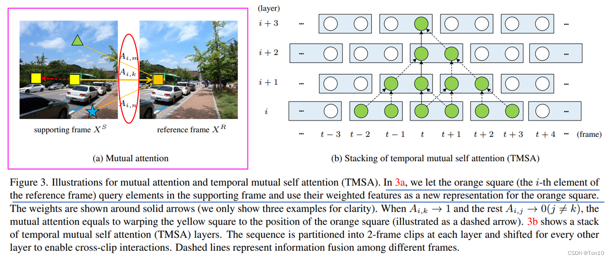
Pictured above (a) It shows 2 Similarity calculation between frames , To calculate the 3 individual $A_{i,m},A_{i,k},A_{i,n}$, Then for $\forall j\ne k(j\le N)$, There are $A_{i,k}>A_{i,j}$, It means that... In the frame is supported $k^{th}$ individual token And reference frame $i^{th}$ individual token It's the most similar . Special , When in addition to $k^{th}$ individual token All but token And the reference frame $i^{th}$ individual token Are very different , There are the following expressions ：
$$\{\begin{array}{l}{A}_{i,k}\to 1,\\ A_{i,j}\to 0,forj\ne k,j\le N\end{array}.\text{\hspace{1em}(5)}$$ Then there is $Y_{i,:}^R=V_{k,:}^S$, This is equivalent to supporting $k^{th}$ individual token Moved to the reference frame $i^{th}$ The position of . This is actually TTVSR The hard attention mechanism in , It is an implicit motion compensation . This kind of hard attention is equivalent to warp, The result is the alignment of the support frame and the reference frame .

Why? MMA It has alignment function ？

The specific explanation is shown in the figure above , Due to the output of new token Is and Query The index of is consistent , Therefore, the output is at the same position as the reference frame token That is, it supports in frame $k^{th}$ Of token Copied over . This duplication is similar to flow-based Aligned copies are very similar , therefore MMA It can be said to be an implicit optical flow estimation +warp The process of .
Note：

1. Then the natural style (5) Not in time , type (4) It becomes soft Version implicit warp The process of .
2. The above two frames are not adjacent frames , But for visual effects , Treat it as two adjacent frames .

Next Change the position of the reference frame and the support frame , Do the equation again (3), We get the second result , We will do the above 2 The fusion of the two results is the final MA Result . Just like self attention ,MA It is also possible to introduce a bull (multi-head) How to do it , Become MMA.

MMA be relative to flow-based Advantages of alignment ：

1. Hard focused MMA The original feature information can be saved directly , It directly copies the target token, It does not involve the operation of interpolation ,flow-based This method inevitably introduces interpolation operation , Some high-frequency information will be lost and it is easy to introduce aliasing artifacts.
2. MMA be based on Transformer, So it doesn't have flow-based be based on CNN So the inductive bias for local correlation , But it also brings benefits ： When 1 individual token If the motion directions of several pixels in the are different ,flow-based Interpolation will be performed during processing , Then finally warp There must be something wrong with the value of a certain pixel ; and MMA Direct replication will not be affected .
3. MMA Belong to one-stage alignment , It's done all at once flow-based Optical flow estimation in alignment +warp2 A process of operations .

MMA It's actually done on the window , We set the window to $(2,\sqrt{N},\sqrt{N})$, be MMA The input is $X\in {\mathbb{R}}^{2\times N\times C}$, If it's self attention , It's right there $2N$ individual token Do your attention , This sum VSRT Time and space attention is the same , and MMA First use torch.chunk take $X$ Split along the time axis 2 Share ——$X_1\in {\mathbb{R}}^{1\times N\times C}、X_2\in {\mathbb{R}}^{1\times N\times C}$, And then execute ：
$$\begin{gathered} X_1\stackrel{warp}{\to }{X}_2, \\ {X}_2\stackrel{warp}{\to }{X}_1. \end{gathered}$$ And will 2 Results can be fused .

$Temporalmutualselfattention$
MMA Will 2 The information of the frames are aligned with each other , But the original characteristic information will be lost , So the author set up self attention MMA To preserve MMA Lost information .MMA The adoption is based on windows Self - attention calculation , and VSRT The same is equivalent to the space-time attention layer . The specific way is to MMA and MSA stay token-embedding Dimensional integration , And then use FC Perform channel reduction .MMA and MSA That's the combination of the two TMSA The attention layer , Then I'll pick up FFN Is complete TMSA modular , The specific expression is as follows ：
$$\begin{gathered} X_1,X_2=Spli{t}_0(LN(X)) \\ {Y}_1,Y_2=MMA(X_1,X_2),MMA(X_2,X_1) \\ {Y}_3=MSA([X_1,X_2]) \\ X=MLP(Conca{t}_2(Conca{t}_1(Y_1,Y_2),Y_3))+X \\ X=MLP(LN(X))+X.\text{\hspace{1em}(6)} \end{gathered}$$

$windowsandshifting-windows$
It can be seen that at present ,MMA The alignment of can only take advantage of adjacent 2 Between frames , It is obviously not enough time to feel the wild , The information available is local , To solve this problem ,VRT use swin-T in shifting The idea of operation , Move the time frame . The specific method is ： Set the window to $(2,8,8)$, Under normal circumstances, the time window moves to half of the window , namely 1, When TMSAG Medium TMSA When it is an odd number of layers , We move the time dimension of the sequence 1 grid , Otherwise it doesn't move , And no matter TMSA Inside, whether or not it moves , Will eventually return to the sequence state before the move .

In this way , After the time axis moves ,$i^{th}$ Of windows Doing it MMA When , Will make use of the previous $2(i-1),i\ge 2$ Characteristic information of the frame . The details are as follows: (b) Shown ：

In order to reduce Transformer because token Too much computation and increasing the range of feature propagation , The author used 3 Windows of dimension and 3 Dimensional shifting-windows, Spatially it is and swin-T Same operation , It's just that there's less to increase the receptive field token Integration mechanism ; In addition, due to VRT Applied to video super division , Therefore, in the time dimension, windows and shifting Window mechanism .

3.3 Parallel Warping

Parallel Warping Is essentially an input sequence $x\in {\mathbb{R}}^{B\times D\times C\times H\times W}$ in 2 Use... In sequence between frames BasicVSR++ Proposed flow-guided DCN Alignment alignment , Do this both forward and backward , When the sequence is finished , Align the results forward and backward, and $x$ Do fusion , And use the full connection layer for channel reduction .

VRL The optical flow used in DCN Alignment and BasicVSR++ It's the same . But I'd like to say it again , As shown in the figure below ：

VRT and VSRT equally , Need to put 2 The adjacent frames of the lattice are aligned with the intermediate frames respectively , Then merge the three .

set up $O_{t-1,t}、O_{t+1,t}$ Namely 2 An optical flow signal ;$\mathcal{W}$ yes flow-based do warp;$X_{t-1}^{{}^{\prime }},X_{t+1}^{{}^{\prime }}$ Is the result of pre alignment ：
$$\{\begin{array}{l}{X}_{t-1}^{{}^{\prime }}=\mathcal{W}(X_{t-1},O_{t-1,t}),\\ X_{t+1}^{{}^{\prime }}=\mathcal{W}(X_{t+1},O_{t+1,t}).\end{array}\text{\hspace{1em}(7)}$$
Next use 1 Several lightweight ones CNN Superimposed network $\mathcal{C}$ To learn the residual part offset and modulation mask：
$$o_{t-1,t},o_{t+1,t},m_{t-1,t},m_{t+1,t}=\mathcal{C}(Concat(O_{t-1,t},O_{t+1,t}),X_{t-1}^{{}^{\prime }},X_{t+1}^{{}^{\prime }}).\text{\hspace{1em}(8)}$$
End use $DCN$ To do it warp, use $\mathcal{D}$ Express , The result of the alignment is ${\hat{X}}_{t-1},{\hat{X}}_{t+1}$：
$$\{\begin{array}{l}{\hat{X}}_{t-1}=\mathcal{D}(X_{t-1},O_{t-1,t}+o_{t-1,t},m_{t-1,t}),\\ {\hat{X}}_{t+1}=\mathcal{D}(X_{t+1},O_{t+1,t}+o_{t+1,t},m_{t+1,t}).\end{array}\text{\hspace{1em}(9)}$$

4 Experiments

4.1 Experimental Setup

①VRT Experimental setup ：

1. Total settings 4 Species scale (stage1~7), about $64\times 64$ Of patch, Set up $64\times 64、32\times 32、16\times 16、8\times 8$ Four resolutions . For each scale setting 8 individual TMSA modular , The top 6 Time windows are 2, after 2 Time windows are 8( For the input sequence is 16 At the frame ) And there is no MMA. The space window is $8\times 8$,head The number of 6. Last group TMSA modular (stage8) Set up 6 individual TMSAG, Each has 4 individual TMSA Module and all are self attention free MMA.
2. about stage1~7,token-embedding The dimension is set to 120, and stage8 Is set to 180.
3. Optical flow estimation uses SpyNet The Internet ( front 2W individual iterations Fixed parameter , The learning rate is set as $5\times 10^{-5}$),FFN Use GRGLU The Internet .
4. batch Set to 8,iterations Set to 30W Time .
5. Use Adam and CA Make optimization , The initial learning rate is set as $4\times 10^{-4}$, And gradually decline .
6. Input patch Choose as $64\times 64$.
7. The experiment involves training 2 Sequence length ——5 and 16, Respectively in 8 Zhang A100 Time consuming 5 and 10 God .

② Data sets ：
The same ones ：REDS、Vimeo-90K. I won't introduce the details , It's all too familiar , Just say it REDS4 yes $clips\{000,011,015,020\}$.

4.2 Video SR

The results of the experiment are as follows ：

The results are as follows ：

1. stay VSRT It has been proved in the paper experiment BasicVSR Weak expressiveness on short sequences , and VRT It can have good expressiveness in both short sequence and long sequence , Especially on short sequences , Because of its better aggregation of local spatial information , So even if the sequence length is short , It can also reconstruct the video better .
2. VRT stay REDS Slightly inferior to BasicVSR++, This is because VRT Only in 16 Train on the frame , The latter is in the 30 Results of training on frame .

---

The visualization results are as follows ：

4.3 Video Deblurring

A little

4.4 Video Denoising

A little

4.5 Ablation Study

$Multi-scale\&Parallelwarping$
To explore multiple scales and PW Influence , The relevant experimental results are as follows ：

The results are as follows ：

1. It can be seen that the richer the scale, the more the performance will be improved , This is because multiscale can guarantee VRT Feature information of multiple resolutions can be used , The larger receptive field can handle the problem of large movement .
2. PW It also brought 0.17dB Performance improvement of .

$TMSA$
To explore TMSA in MMA and MSA Influence , The relevant experimental results are as follows ：

The results are as follows ：

1. It's just MMA But not MSA You can't , because MMA The original feature information will be lost .
2. In addition to MMA and MSA Under the circumstances ,VRT The expressiveness of has been improved .

$Windowsize$
At each scale TMSAG in , The author will follow 2 individual TMSA The time receptive field increases , This is to further increase the ability to capture feature information in a long range of sequences . The relevant experimental results are as follows ：

The results are as follows ：

1. Time window from 1 To 2 about PSNR There's a limit to the promotion of , But to 8 When , There are still some improvements , Therefore, the window size of the last time dimension is set 8.

5 Conclusion

1. This paper introduces a method based on Vision-Transformer Of Parallelized video hyperfractionation model ——VRT.VRT Based on multi-scale (multi-scale) To do the alignment under different resolutions , At the same time, different local feature information can be extracted from different scales .VRT The overall architecture is divided into feature extraction and SR The reconstruction 2 Parts of , It can be applied to a variety of video recovery tasks .
2. VRT draw swin-T Thought , On both spatial and temporal scales shifting, So as to separate It ensures the clustering of spatial local correlations and the ability of long sequences to capture global correlations .
3. VRT It introduces MMA, A mechanism of mutual attention , Different from self attention, it is used to extract spatiotemporal features ,MMA Can be used to do one-stage Feature alignment for . Besides MMA and MSA Are based on windows , In addition to better extraction of local information, it can also reduce the amount of calculation of similarity .
4. VRT learn BasicVSR++ Guided by optical flow DCN Alignment mode , Yes VSRT in flow-based Alignment makes improvements , Thus, the Parallel Warping modular .