Methods for converting one-dimensional data (sequence) into two-dimensional data (image) GAFS, MTF, recurrence plot, STFT

Methods for converting one-dimensional sequence data into two-dimensional image data detailed comprehensive

• One 、 background
• Two 、 Methods to introduce
• • Grameen angle field GAFs
  • • principle
    • Implementation steps
    • Invoke the sample
  • Markov transition field MTF
  • • principle
    • Implementation steps
    • Invoke the sample
  • Recursive graph Recurrence Plot
  • • principle
    • Invoke the sample
  • The short-time Fourier transform STFT
  • principle
  • Implementation steps
  • Invoke the sample
• References
• summary

One 、 background

Although the deep learning method (1D CNN, RNN, LSTM etc. ) It can directly process one-dimensional data , But the current deep learning methods mainly deal with two-dimensional structure data , Especially in computer vision CV And natural language processing NLP field , Various methods emerge in endlessly . therefore , If one-dimensional sequence data can be transformed into two-dimensional data ( Images ) data , Can be directly combined with CV as well as NLP Domain approach , Isn't it very interesting ！

Two 、 Methods to introduce

Grameen angle field GAFs

principle

take The zoom After 1D Sequence data from Rectangular coordinate system The switch to Polar coordinate system , Then by considering the angles between different points and / Difference to identify... At different points in time Time relevance . It depends on whether the angle is sum or difference , Yes There are two ways to achieve ：GASF( Make an angle and ), GADF( Corresponding to the angle difference ).

Implementation steps

Step 1： The zoom , Scale the data range to [-1,1] perhaps [0, 1], The formula is as follows ：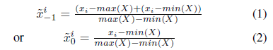

Step 2: Convert the scaled sequence data to polar coordinate system , That is, the value is regarded as the cosine value of the included angle , Time stamp is regarded as radius , The formula is as follows ：

notes ： If the data scaling range is [-1, 1], Then the angle range after conversion is [0, π pi π]; If the zoom range is [0, 1], Then the angle range after conversion is [0, π pi π/2].
Step 3:

You can see , Final GASF and GADF The calculation of is transformed into a rectangular coordinate system “ similar ” Operation of inner product .

The efficiency problem ： For length is n The sequence data of , Converted GAFs Size is [n, n] Matrix , May adopt PAA( Piecewise aggregation approximation ) First reduce the sequence length , Then in the conversion . So-called PAA Namely ： Segment the sequence , Then, the subsequence in each segment is compressed into a numerical value by averaging , Easy ！

Invoke the sample

Python tool kit pytl We have provided API, in addition , The author implements the code by himself , Want to see the implementation details and get more test cases , But from my link obtain .

'''
EnvironmentPython 3.6,  pyts: 0.11.0, Pandas: 1.0.3
'''
from mpl_toolkits.axes_grid1 import make_axes_locatable
from pyts.datasets import load_gunpoint
from pyts.image import GramianAngularField
# call API
X, _, _, _ = load_gunpoint(return_X_y=True)
gasf = GramianAngularField(method='summation')
X_gasf = gasf.transform(X)
gadf = GramianAngularField(method='difference')
X_gadf = gadf.transform(X)

plt.figure()
plt.suptitle('gunpoint_index_' + str(0))
ax1 = plt.subplot(121)
ax1.plot(np.arange(len(rescale(X[k][:]))), rescale(X[k][:]))
plt.title('rescaled time series')
ax2 = plt.subplot(122, polar=True)
r = np.array(range(1, len(X[k]) + 1)) / 150
theta = np.arccos(np.array(rescale(X[k][:]))) * 2 * np.pi  # radian -> Angle

ax2.plot(theta, r, color='r', linewidth=3)
plt.title('polar system')
plt.show()

plt.figure()
plt.suptitle('gunpoint_index_' + str(0))
ax1 = plt.subplot(121)
plt.imshow(X_gasf[k])
plt.title('GASF')
divider = make_axes_locatable(ax1)
cax = divider.append_axes("right", size="5%", pad=0.2) # Create an axes at the given *position*=right with the same height (or width) of the main axes
plt.colorbar(cax=cax)

ax2 = plt.subplot(122)
plt.imshow(X_gadf[k])
plt.title('GASF')
divider = make_axes_locatable(ax2)
cax = divider.append_axes("right", size="5%",
                          pad=0.2)  # Create an axes at the given *position*=right with the same height (or width) of the main axes
plt.colorbar(cax=cax)
plt.show()

The results are shown in the following figure ：
Scaled sequence data and representation in polar coordinate system ：

Converted GASF and GADF:

---

Markov transition field MTF

principle

be based on 1 Order Markov chain , Because the Markov transition matrix is not sensitive to the time dependence of the sequence , Therefore, the author puts forward the so-called MTF.

Implementation steps

Step 1: First, sequence data ( The length is n) According to its value range, it is divided into Q individual bins ( Similar to quantile ), Every data point i Belong to a unique qi ( ∈ in ∈ {1,2, …, Q}).
Step 2: Construct Markov transition matrix W, The matrix size is ：[Q, Q], among W[i,j] from qi The data in is qj The frequency immediately adjacent to the data in , Its calculation formula is as follows ：
w i , j = ∑ x ∈ q i , y ∈ q j , x + 1 = y 1 / ∑ j = 1 Q w i , j w_{i,j}=sum_{ orall x in q_{i}, y in q_{j},x+1=y}1/sum_{j=1}^{Q}w_{i,j} wi,j=∑x∈qi,y∈qj,x+1=y1/∑j=1Qwi,j
Step 3: Construct Markov transition field M, The matrix size is ：[n, n], M[i,j] The value of is W[qi, qj]

The efficiency problem ： Reason and GAFs similar , In order to improve efficiency , Try to reduce M The size of the , Ideas and PAA similar , take M Gridding , Then the subgraphs in each grid are replaced by their average values .

Invoke the sample

Python tool kit pytl We have provided API,API Interface reference ：https://pyts.readthedocs.io/en/latest/generated/pyts.image.MarkovTransitionField.html. in addition , The author implements the code by himself , Want to see the implementation details and get more test cases , But from my github link obtain .

'''
EnvironmentPython 3.6,  pyts: 0.11.0, Pandas: 1.0.3
'''
from mpl_toolkits.axes_grid1 import make_axes_locatable
from pyts.datasets import load_gunpoint
from pyts.image import MarkovTransitionField
## call API
X, _, _, _ = load_gunpoint(return_X_y=True)
mtf = MarkovTransitionField()
fullimage = mtf.transform(X)

# downscale MTF of the time series (without paa) through mean operation
batch = int(len(X[0]) / s)
patch = []
for p in range(s):
    for q in range(s):
        patch.append(np.mean(fullimage[0][p * batch:(p + 1) * batch, q * batch:(q + 1) * batch]))
# reshape
patchimage = np.array(patch).reshape(s, s)

plt.figure()
plt.suptitle('gunpoint_index_' + str(k))
ax1 = plt.subplot(121)
plt.imshow(fullimage[k])
plt.title('full image')
divider = make_axes_locatable(ax1)
cax = divider.append_axes("right", size="5%", pad=0.2)
plt.colorbar(cax=cax)

ax2 = plt.subplot(122)
plt.imshow(patchimage)
plt.title('MTF with patch average')
divider = make_axes_locatable(ax2)
cax = divider.append_axes("right", size="5%", pad=0.2)
plt.colorbar(cax=cax)
plt.show()

The result is shown in the figure ：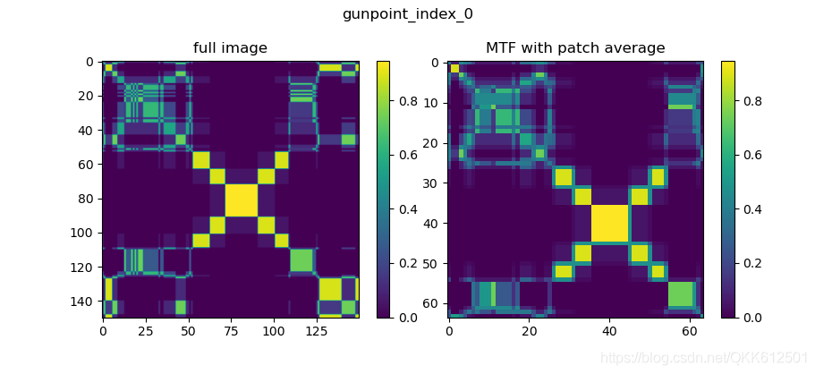

---

Recursive graph Recurrence Plot

Recursive graph (recurrence plot,RP) Is to analyze the periodicity of time series 、 An important method of chaos and nonstationarity , It can reveal the internal structure of time series , Give information about similarity 、 A priori knowledge of information and predictability , Recursive graph is especially suitable for short time series data , It can test the stationarity of time series 、 Internal similarity .

principle

A recursive graph is an image that represents the distance between tracks extracted from the original time series
Given time series data : ( x 1 , … , x n ) (x_1, ldots, x_n) (x1,…,xn), The extracted track is ：
x i = ( x i , x i + τ , … , x i + ( m 1 ) τ ) , i ∈ { 1 , … , n ( m 1 ) τ } ec{x}_i = (x_i, x_{i + au}, ldots, x_{i + (m - 1) au}), quad orall i in {1, ldots, n - (m - 1) au } x i=(xi,xi+τ,…,xi+(m1)τ),i∈{1,…,n(m1)τ}
among ： m m m Is the dimension of the trajectory , τ au τ Is delay . Recursive graph R Is the pairwise distance between tracks , The calculation is as follows ：
R i , j = Θ ( ε ∥ x i x j ∥ ) , i , j ∈ { 1 , … , n ( m 1 ) τ } R_{i, j} = Theta(arepsilon - | ec{x}_i - ec{x}_j |), quad orall i,j in {1, ldots, n - (m - 1) au } Ri,j=Θ(ε∥x ix j∥),i,j∈{1,…,n(m1)τ}
among , Θ Theta Θ by Heaviside function , and ε arepsilon ε It's the threshold .

Invoke the sample

'''
EnvironmentPython 3.6,  pyts: 0.11.0, Pandas: 1.0.3
'''
from mpl_toolkits.axes_grid1 import make_axes_locatable
from pyts.datasets import load_gunpoint
from pyts.image import RecurrencePlot

X, _, _, _ = load_gunpoint(return_X_y=True)
rp = RecurrencePlot(dimension=3, time_delay=3)
X_new = rp.transform(X)
rp2 = RecurrencePlot(dimension=3, time_delay=10)
X_new2 = rp2.transform(X)
plt.figure()
plt.suptitle('gunpoint_index_0')
ax1 = plt.subplot(121)
plt.imshow(X_new[0])
plt.title('Recurrence plot, dimension=3, time_delay=3')
divider = make_axes_locatable(ax1)
cax = divider.append_axes("right", size="5%", pad=0.2)
plt.colorbar(cax=cax)

ax1 = plt.subplot(122)
plt.imshow(X_new2[0])
plt.title('Recurrence plot, dimension=3, time_delay=10')
divider = make_axes_locatable(ax1)
cax = divider.append_axes("right", size="5%", pad=0.2)
plt.colorbar(cax=cax)
plt.show()

The result is shown in Fig. ：

---

The short-time Fourier transform STFT

STFT It can be regarded as a way to quantify the time-varying frequency and phase content of non-stationary signals ..

principle

By adding window functions （ The length of the window function is fixed ）, First, the time domain signal is windowed , The original time domain signal is divided into multiple segments by sliding window , And then, for each segment FFT Transformation , Thus the time spectrum of the signal is obtained （ Time domain information is preserved ）.

Implementation steps

Suppose the length of the sequence is T T T, τ au τ Is the window length , s s s Is the sliding step size ,W Representation window function , be STFT It can be calculated as ：

S T F T ( τ , s ) ( X ) [ m , k ] = ∑ t = 1 T X [ t ] W ( t s m ) e x p { j 2 π k / τ ( t s m ) } STFT^{( au,s)}(X)_{[m,k]}=sum_{t=1}^{T}X_{[t]} cdot W(t-sm)cdot exp{-j2pi k / au cdot (t-sm)} STFT(τ,s)(X)[m,k]=∑t=1TX[t]W(tsm)exp{j2πk/τ(tsm)}

Transformed STFT Size is ：[M, K], M Represents the time dimension ,K Represents the frequency amplitude ( Plural form ), For convenience , hypothesis s = τ s= au s=τ, That is, there is no overlap between windows , be
M = T / τ M=T/ au M=T/τ,
K = τ K =lfloor au floor K=τ/2 + 1

notes ： Compared with DFT, STFT To some extent, it helps us restore the time resolution , However, there is a trade-off between achievable temporal resolution and frequency , That's what's called The principle of uncertainty . say concretely , Width of window （ τ au τ） The bigger it is , The higher the frequency domain resolution , Accordingly , The lower the time domain resolution ; Width of window （ τ au τ） The smaller it is , The lower the frequency-domain resolution , Accordingly , The higher the time domain resolution .

Invoke the sample

python package scipy Provide STFT Of API, For details of the official documents, see ：https://docs.scipy.org/doc/scipy/reference/generated/scipy.signal.stft.html

scipy.signal.stft(x,fs = 1.0,window =‘hann’,nperseg = 256,noverlap = None,nfft = None,detrend = False,return_oneside = True,boundary
=‘zeros’,padded = True,axis = -1 ）

Parameter interpretation ：
x： Time domain signal ;
fs： Sampling frequency of the signal ;
window： Window function ;
nperseg： Window function length ;
noverlap： Overlap length of adjacent windows , The default is 50%;
nfft： FFT The length of , The default is nperseg. If it is greater than nperseg Will automatically zero fill ;
return_oneside ： True Returns the real part of a complex number ,None Returns the complex number .
Sample code ：

"""
@author: masterqkk, [email protected]
Environment:
    python: 3.6
    Pandas: 1.0.3
    matplotlib: 3.2.1
"""
import pickle
import numpy as np
import matplotlib.pyplot as plt
import scipy.signal as scisig
from mpl_toolkits.axes_grid1 import make_axes_locatable
from pyts.datasets import load_gunpoint

if __name__ == '__main__':
    X, _, _, _ = load_gunpoint(return_X_y=True)

    fs = 10e3  # sampling frequency
    N = 1e5  # 10 s 1signal
    amp = 2 * np.sqrt(2)
    time = np.arange(N) / float(fs)
    mod = 500 * np.cos(2 * np.pi * 0.25 * time)
    carrier = amp * np.sin(2 * np.pi * 3e3 * time + mod)
    noise_power = 0.01 * fs / 2
    noise = np.random.normal(loc=0.0, scale=np.sqrt(noise_power), size=time.shape)
    noise *= np.exp(-time / 5)
    x = carrier + noise  # signal with noise

    per_seg_length = 1000 # window length
    f, t, Zxx = scisig.stft(x, fs, nperseg=per_seg_length, noverlap=0, nfft=per_seg_length, padded=False)
    print('Zxx.shaope: {}'.format(Zxx.shape))  

    plt.figure()
    plt.suptitle('gunpoint_index_0')
    ax1 = plt.subplot(211)
    ax1.plot(x)
    plt.title('signal with noise')

    ax2 = plt.subplot(212)
    ax2.pcolormesh(t, f, np.abs(Zxx), vmin=0, vmax=amp)
    plt.title('STFT Magnitude')
    ax2.set_ylabel('Frequency [Hz]')
    ax2.set_xlabel('Time [sec]')
    plt.show()

Running results ：
obtain STFT The resulting size is ：
Zxx.shaope: (501, 101), The number of frequency components is 1000 lfloor 1000 floor 1000/2 + 1 = 501, The length of the window fragment is 1e5/1000 + 1=101 ( Here should be a pad)

References

1.Imaging Time-Series to Improve Classification and Imputation
2.Encoding Time Series as Images for Visual Inspection and Classification Using Tiled Convolutional Neural Networks
3.J.-P Eckmann, S. Oliffson Kamphorst and D Ruelle, “Recurrence Plots of Dynamical Systems”. Europhysics Letters (1987)
4.Stoica, Petre, and Randolph Moses,Spectral Analysis of Signals, Prentice Hall, 2005
5.https://laszukdawid.com/tag/recurrence-plot/

summary

Finally, a link to download the time series data set is attached ：http://www.cs.ucr.edu/~eamonn/time_series_data/, It contains almost all current data sets in this field .
I hope I can help you , To be continued . Welcome to exchange ：[email protected]